Experiment 1 Progress

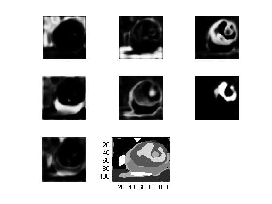
For our progress on the first experiment, we are able to compute the following probability:

P(pixel p belongs in label i)

For each pixel p in our test image:

 

 Given our manual photoshop segmentation with labels i (1-7)

 

The following images represent the probability that each pixel belongs to the labels 1-7. The last image in each chart segments the image by assigning the pixel to the label with the highest probability (Note this does not incorporate the k-means algorithm yet)

 

sigma = 0.05

bin count = 15

Small sigma causes high contrast between segments

sigma = 0.2

bin_count = 15

Larger sigma causes less contrast between segments

sigma = 0.2

bin count = 40

Larger bin count causes more noise

In the following examples, we computed the histogram of the window around each pixel, which smoothed out the segmentation

sigma = 0.3

bin count = 15

window size = 3

sigma = 0.3

bin count = 15

window size =11

Larger window size increased smoothing, but also caused regions to spill over more

------

We are also planning to follow up on what Professor Belongie said in class about conditional random fields. 

We intend to read the following links. 

http://www.cs.rochester.edu/~ardis/sept21.pdf

http://www.cis.upenn.edu/~pereira/papers/crf.pdf