MultiBoost and finalizing training data

We were able to compile and run MultiBoost with a basic example, and import the results into Matlab. With Karmen's help we we're able to understand the strong classifier produced. We are still in the process of creating features for our superpixels, which we will plugin to MultiBoost to get a classifier from superpixels to their 3d surface normal.

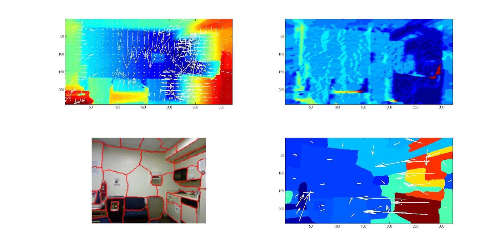
We were able to fix the average 3D surface normals assigned to superpixels. The following pictures show surface normal classification in our training set. The normals are divided into classes based on the their angle in the xy and xz planes.

 

1) Depth map with 3D surface normals overlayed

2) Per pixel surface normal classes (128 total classes)

3) Finescale superpixel segmentation

4) Finescale superpixel classes (128 total classes) with 3D surface normals overlayed

1) Depth map with 3D surface normals overlayed

2) Per pixel surface normal classes (16 total classes)

3) Larger superpixel segmentation

4) Larger superpixel classes (16 total classes) with 3D surface normals overlayed

1) Depth map with 3D surface normals overlayed

2) Per pixel surface normal classes (128 total classes)

3) Finescale superpixel segmentation

4) Finescale superpixel classes (128 total classes) with 3D surface normals overlayed

1) Depth map with 3D surface normals overlayed

2) Per pixel surface normal classes (16 total classes)

3) Larger superpixel segmentation

4) Larger superpixel classes (16 total classes) with 3D surface normals overlayed


 One observation in all of these is that there appears to be somewhat of a checkerboard pattern of the classes assigned to superpixels on a single surface (especially on the left wall of the second image).

This happens when the surface normal is right on the border between two classes.

For example, let's say the xy angle for class 1 is between 0 and 45, and the xy angle for class 2 is between 45 and 90.  If we have a wall whose estimated surface normals have an xy angle that varies between 40 and 50, the surface normals are still pointing approximately in one direction, but it bounces back and forth between these two classes).

We should still be able to exploit the fact that certain classes are closely related and can be clumped together in the final segmentation process.

Extracting surface normals from depth maps (continued)

Using the method described in sections 3.2 and 3.3 from this surface reconstruction: Surface Reconstruction from Unorganized Points, we were able to write a Matlab script to extract decent 3d normals from the point cloud given by the NYU dataset. Viewing in Meshlab with a light, the scene is shaded properly:

The following images shows results for our attempts to classify different regions of an image according to their 3D surface orientation. We're currently dividing the possible orientations into 64 discrete classes.

(Left to Right)
1) 3D normals flattened on the 2d depth map (dividing x and y component by the z component)
2) Classification of each pixel normal according to 64 possible classes

3) Superpixels
4) Classification of each superpixel according to average normal (has problems)

Once a few issues are fixed, we will have a training data set where each superpixel has a surface position and orientation. Our next step will be to develop a classifier to take a superpixel patch and output a normal and position.

Extracting surface normals from depth maps

For the direction of our project, we want to identify geometric classes in the scene as well as object labels. We can use the depth maps from the NYU dataset to train geometric classes for objects based on their surface normals, which we can extract from the depth map. We will follow closely the methods used by Hoiem et al. in the following paper: Geometric Context from a Single Image.

The following is from a sample image in the NYU dataset of a room with a depth map, and object labels.

(From left to right).  

1) RGB image 

2) Depth map with the vector field of gradients, which gives us the 3D orientation of the surface

3) Magnitude of the gradient divided by the depth value squared, and with histogram normalization

4) Object labels from dataset

5) Superpixels segmentation

Close up of the depth map with gradients.  We are hoping to extract the surface normal of different surfaces in the scene from the 2D gradient of the depth map. The direction of the gradient should indicate the X and Y components of the surface normal, while the magnitude should give us some indication of the Z component of the normal.

 

(Left to right)

1) Depth map image

2) Raw gradient magnitude

3) Gradient magnitude after applying histogram equalization. For surfaces that recede into the scene, the gradient magnitude increases. This represents a problem, because for a flat surface, the surface normal should remain consistent throughout (otherwise it looks like the surface is curved).

4) After dividing the gradient magnitude by the depth-value squared, the gradient magnitude remains more consistent across flat surfaces receding into the scene

Here is a more problematic image

For this image, dividing by the depth squared did not fix the problem of the gradient magnitude remaining consistent throughout the flat surface of the hallway.

Another problem with using the depth map gradient to determine the surface normal is that object edges cause spikes in the gradient magnitude, and they don't necessarily represent surfaces (like the object on the wall near the bottom of the image)

We are most likely going to be using some form of Adaboost to develop our classifier.

Useful matlab commands for large datasets

We were finally able to load the dataset from NYU using the following matlab commands. These may be useful for anyone using datasets with very large matlab files that you can't load all at once into memory.

%% Partial Reading and Writing of MAT Files

%% Looking at what is in the file
% You can use the following to to see what variables are available in your MAT-file

whos -file myBigData

%%  Creating a MAT-File object
% Create a object that corresponds to a MAT-File

matObj = matfile('myBigData.mat');

%% Accessing Variables
% Now you can access variables in the MAT-file as properties of |matObj|,
% with dot notation. This is similar to how you access the fields of
% structures in MATLAB.

loadedData = matObj.X(1:4,1:4);
disp(loadedData)

Superpixels and dataset from NYU

We we're able to get the superpixels Matlab code working from this site by following this tutorial. We ran it on a sample indoor scene:

We also found a dataset from a research group in NYU of indoor scenes with labeled masks as well as depth-maps obtained from the Kinect. We weren't able to load the data into Matlab yet, probably because it couldn't handle the file size (4 gigs). However, we were able to contact the author Nathan Silberman via email, who graciously offered to split up the data into separate files for us.

The paper corresponding to this dataset made use of SIFT feature detectors, we tested and got running an implementation of SIFT here. We're debating whether or not to include this in our algorithm.

What to Do Next

We've decided to experiment with superpixels for our project.

We are looking into using the following code:

Superpixel code

As you can see from the baseball player pictures in the aforementioned link, superpixels divide an image into segments along edge boundaries near perfectly. The problem then simplifies into clustering superpixels into larger segments according to labels.

We are also looking very closely at the following paper on hierarchical region segmentation:

Context by Region Ancestry

It is based on work from UC Berkeley's computer vision research group on contour image segmentation:

Berkeley Contour Segmentation