Superpixel Classification and 3D Projection

We've finalized the pipeline to go from an RGB image of an indoor scene to a 3D popup model:

We are given an RGB image divided up into superpixels. We make the assumption that each superpixel represents approximately a flat surface in 3D space. We identify the plane in space the surface lies on, and then project the 2D pixels onto that plane in 3D.

We are able to infer the approximate 3D surface normal and position of a superpixel in our dataset using the depth data from the Kinect. Given that, we can classify each superpixel according to some orientation and location.

Classifier

We assign an orientation class (based on the estimated 3D surface normal) and a depth subclass. The 3D surface normal defines a plane somewhere in space. The depth subclass gives the distance of the plane from the origin.

We have 7 orientation classes. Because the camera in our training set rarely looks up or down, the floor and ceiling always have the same orientation, so we only need one class for each of them. However, walls in the scene can have any number of orientations, so we are currently giving 5 total classes for walls.
  
Orientation Classes       Surface Normal        
1 Up                               [0 1 0]                     (floors, tables, chair seats)
2 Down                          [0 -1 0]                    (ceiling)
3 Right                           [1 0 0]                     (walls)
4 Right-Center               [1 0 -1]
5 Center                         [0 0 -1]
6 Left-Center                 [-1 0 -1]
7 Left                             [-1 0 0]

We have 10 total location subclasses for each orientation class. A location subclass gives us the distance from the plane to the origin, which tells us where the surface is in 3D space.

Features

To classify each superpixel, we are currently using a set of basic descriptors:

RGB mean                                                                           XY mean                                                                              
DOG (Difference of Gaussians) mean                                
Area                                                                                     
DOG histogram (6 bins)                                                      
RGB histogram (6 bins each)                                              

The total number of dimensions of the feature vector is 31

We will then plug our feature vectors per superpixel and their classes into MultiBoost to get a single strong learner for the orientations, and then for each orientation we have a separate strong learner to get the location class.

We believe finding the location is a harder problem than finding the orientation. So it makes sense to make the location classification conditioned on the type of surface. The location of the 3D plane for ceiling and floors stays constant for most of the training images. We believe we will be able to classify ceiling and floors with higher confidence then walls.

Stitching Algorithm

The next step is to use a stitching algorithm that will iteratively perturb the superpixel surface normals and orientations from their estimated value, with the goal of piecing them together so they fit in 3D space. We will update this blog post to discuss this algorithm in more detail at a later time

 

(Left to right)
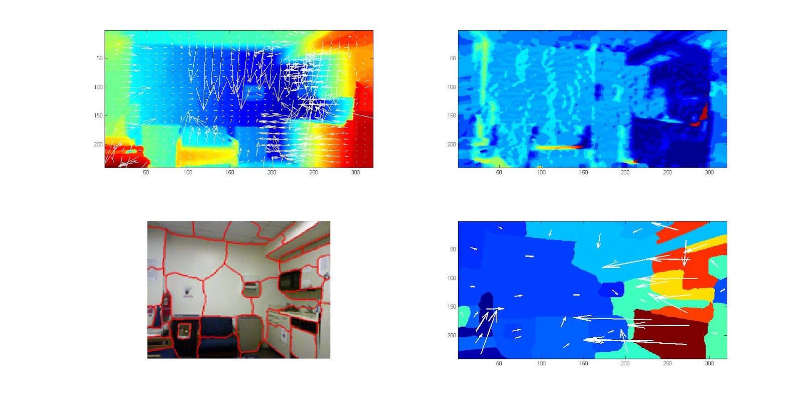
1) Original image divided into 40 superpixels
2) Depth map with per-pixel orientations
3) Superpixel location classes
4) Superpixel orientation classes


For the following images we show the point cloud result from projecting the superpixels onto their plane in 3D space. We show both the projection of the actual 3D location and normal estimated from the Kinect, and also the classified 3D location and normal.

Projection using actual normal/location(superpixel resolution 40)

Projection using the classified normal/location (superpixel resolution 40)


The following images use a higher superpixel resolution of 200. Using a higher superpixel resolution, the popup model more closely resembles the actual model. However, this will also increase the computational complexity of our stitching algorithm (will be discussed later)

Projection using the actual normal/location (superpixel resolution 200)
 

Projection using the classified normal/location (superpixel resolution 200)


Finally, the highest superpixel resolution (1094):

Projection using the actual normal/location (superpixel resolution 1094)

Projection using the classified normal/location (superpixel resolution 1094)

MultiBoost and finalizing training data

We were able to compile and run MultiBoost with a basic example, and import the results into Matlab. With Karmen's help we we're able to understand the strong classifier produced. We are still in the process of creating features for our superpixels, which we will plugin to MultiBoost to get a classifier from superpixels to their 3d surface normal.

We were able to fix the average 3D surface normals assigned to superpixels. The following pictures show surface normal classification in our training set. The normals are divided into classes based on the their angle in the xy and xz planes.

 

1) Depth map with 3D surface normals overlayed

2) Per pixel surface normal classes (128 total classes)

3) Finescale superpixel segmentation

4) Finescale superpixel classes (128 total classes) with 3D surface normals overlayed

1) Depth map with 3D surface normals overlayed

2) Per pixel surface normal classes (16 total classes)

3) Larger superpixel segmentation

4) Larger superpixel classes (16 total classes) with 3D surface normals overlayed

1) Depth map with 3D surface normals overlayed

2) Per pixel surface normal classes (128 total classes)

3) Finescale superpixel segmentation

4) Finescale superpixel classes (128 total classes) with 3D surface normals overlayed

1) Depth map with 3D surface normals overlayed

2) Per pixel surface normal classes (16 total classes)

3) Larger superpixel segmentation

4) Larger superpixel classes (16 total classes) with 3D surface normals overlayed


 One observation in all of these is that there appears to be somewhat of a checkerboard pattern of the classes assigned to superpixels on a single surface (especially on the left wall of the second image).

This happens when the surface normal is right on the border between two classes.

For example, let's say the xy angle for class 1 is between 0 and 45, and the xy angle for class 2 is between 45 and 90.  If we have a wall whose estimated surface normals have an xy angle that varies between 40 and 50, the surface normals are still pointing approximately in one direction, but it bounces back and forth between these two classes).

We should still be able to exploit the fact that certain classes are closely related and can be clumped together in the final segmentation process.

Extracting surface normals from depth maps (continued)

Using the method described in sections 3.2 and 3.3 from this surface reconstruction: Surface Reconstruction from Unorganized Points, we were able to write a Matlab script to extract decent 3d normals from the point cloud given by the NYU dataset. Viewing in Meshlab with a light, the scene is shaded properly:

The following images shows results for our attempts to classify different regions of an image according to their 3D surface orientation. We're currently dividing the possible orientations into 64 discrete classes.

(Left to Right)
1) 3D normals flattened on the 2d depth map (dividing x and y component by the z component)
2) Classification of each pixel normal according to 64 possible classes

3) Superpixels
4) Classification of each superpixel according to average normal (has problems)

Once a few issues are fixed, we will have a training data set where each superpixel has a surface position and orientation. Our next step will be to develop a classifier to take a superpixel patch and output a normal and position.

Extracting surface normals from depth maps

For the direction of our project, we want to identify geometric classes in the scene as well as object labels. We can use the depth maps from the NYU dataset to train geometric classes for objects based on their surface normals, which we can extract from the depth map. We will follow closely the methods used by Hoiem et al. in the following paper: Geometric Context from a Single Image.

The following is from a sample image in the NYU dataset of a room with a depth map, and object labels.

(From left to right).  

1) RGB image 

2) Depth map with the vector field of gradients, which gives us the 3D orientation of the surface

3) Magnitude of the gradient divided by the depth value squared, and with histogram normalization

4) Object labels from dataset

5) Superpixels segmentation

Close up of the depth map with gradients.  We are hoping to extract the surface normal of different surfaces in the scene from the 2D gradient of the depth map. The direction of the gradient should indicate the X and Y components of the surface normal, while the magnitude should give us some indication of the Z component of the normal.

 

(Left to right)

1) Depth map image

2) Raw gradient magnitude

3) Gradient magnitude after applying histogram equalization. For surfaces that recede into the scene, the gradient magnitude increases. This represents a problem, because for a flat surface, the surface normal should remain consistent throughout (otherwise it looks like the surface is curved).

4) After dividing the gradient magnitude by the depth-value squared, the gradient magnitude remains more consistent across flat surfaces receding into the scene

Here is a more problematic image

For this image, dividing by the depth squared did not fix the problem of the gradient magnitude remaining consistent throughout the flat surface of the hallway.

Another problem with using the depth map gradient to determine the surface normal is that object edges cause spikes in the gradient magnitude, and they don't necessarily represent surfaces (like the object on the wall near the bottom of the image)

We are most likely going to be using some form of Adaboost to develop our classifier.

Useful matlab commands for large datasets

We were finally able to load the dataset from NYU using the following matlab commands. These may be useful for anyone using datasets with very large matlab files that you can't load all at once into memory.

%% Partial Reading and Writing of MAT Files

%% Looking at what is in the file
% You can use the following to to see what variables are available in your MAT-file

whos -file myBigData

%%  Creating a MAT-File object
% Create a object that corresponds to a MAT-File

matObj = matfile('myBigData.mat');

%% Accessing Variables
% Now you can access variables in the MAT-file as properties of |matObj|,
% with dot notation. This is similar to how you access the fields of
% structures in MATLAB.

loadedData = matObj.X(1:4,1:4);
disp(loadedData)

Superpixels and dataset from NYU

We we're able to get the superpixels Matlab code working from this site by following this tutorial. We ran it on a sample indoor scene:

We also found a dataset from a research group in NYU of indoor scenes with labeled masks as well as depth-maps obtained from the Kinect. We weren't able to load the data into Matlab yet, probably because it couldn't handle the file size (4 gigs). However, we were able to contact the author Nathan Silberman via email, who graciously offered to split up the data into separate files for us.

The paper corresponding to this dataset made use of SIFT feature detectors, we tested and got running an implementation of SIFT here. We're debating whether or not to include this in our algorithm.

What to Do Next

We've decided to experiment with superpixels for our project.

We are looking into using the following code:

Superpixel code

As you can see from the baseball player pictures in the aforementioned link, superpixels divide an image into segments along edge boundaries near perfectly. The problem then simplifies into clustering superpixels into larger segments according to labels.

We are also looking very closely at the following paper on hierarchical region segmentation:

Context by Region Ancestry

It is based on work from UC Berkeley's computer vision research group on contour image segmentation:

Berkeley Contour Segmentation

Planning out rest of the project

We've completed our first experiment, and established the framework for our algorithm, which boils down to computing the following probability:

So far we have just used an unigram model based on color histograms to determine these probabilities. We want to add bigram model for spatial relationships between segments. In addition, we also want to incorporate a parse grammar of objects that models contextual relationships between segments.

We will need to assign weights to each model so that the total probability adds up to 1. We are still researching exactly how to learn what these ideal weights should be, we are hoping something like a CRF model will do the trick, or we can just play around with different values. Here's one potential example:

Feature          Unigram          Bigram
Color                  0.2                   0
Centroid              0                   0.2
Area                   0.05               0.2
Context              0.15                 0.2

For contextual relationships, we intend to use a parse grammar similar to the one described here

For ours, we would use segments instead of lines as the elements of the grammar. Ideally, we would like our grammar to represent the 3D geometry of the scene (as in the link above), but to start we will probably just identify some basic labels:

    Foreground                                      Background

       /           \                                     /              |          \

  table        chair                          wall         ceiling    floor

  /     \           /     \                          /    \                           \
legs  top    legs  top               door   window             carpet


Training data - need to figure this out

1) We can create our own training data from simple indoor scenes. For each image, we will have a manually segmented image for each level in the parse tree

If we construct our own data, how many images will we need for our training data?

2) Find something online? We're not sure if anything like what we've described exists.

How to split and merge clusters? (some ideas)

Ideally, we want our algorithm to "find" new objects in the scene, based on its current understanding of the scene. This involves increasing or decreasing the number of segments at each iteration, eventually converging to the proper amount.

For example, given clusters A-G, and labels table and chair. Let's say we know with high probability that cluster A is label 'table', and further we know from contextual relationships that if we see label 'table', then we should see label 'chair' nearby. 

If none of the nearby clusters correspond to a chair, (that is, the probability of P(B or C or D or E or F or G = 'chair' | A = 'table') is really low), then we split one of the clusters (increase k), to try to find a cluster with label 'chair'. Ideally, we want to split the cluster that we have the lowest confidence in its labels.

We split the cluster where we expect the part/object to be (using computer vision techniques, we know generally where it should be).

We merge clusters when they are empty, really small.

Experiment 1 Results

We completed our initial experiment to segment an image with a modified version of k-means by using the histograms for each label from the manual segmentation.

 Here are the results for one run, we have colored the segments according to the highest probable label.

The following table shows the final probabilities assigned to each cluster. 

					Label
Cluster	Pixel Count	1	2	3	4	5	6	7
A	4359	0.9854*	0.0023	0.0003	0.0063	0.0034	0.0002	0.002
B	2589	0.0002	0.0001	0.0002	0	0	0.9994	0
C	2758	0.0039	0.9592	0.0077	0.0003	0.0284	0.0001	0.0003
D	1465	0.3841*	0.2337	0.2917	0.0045	0.0522	0.0282	0.0056
E	220	0.1431*	0.1429	0.1429	0.1428	0.1429	0.143	0.1425
F	1114	0.0178	0.001	0.0019	0.5741	0.0181	0	0.387
G	264	0.0004	0.0125	0.8674	0.0002	0.1183	0.0006	0.0007

 Some interesting observations:
* Clusters A, D and E were assigned the same label
* Clusters E and G have very low pixel counts
* Labels 5 and 7 were not assigned to any cluster.

Need to have some mechanism to deal with clusters that have very low pixel counts


 Here are some more runs comparing our modified K-means with normal k-means. On average, our modified version does segment the image closer to the target segmentation, but there is plenty of room for improvement.

At this point we will start designing the parse tree for slightly more complicated indoor scenes, as well as a bigram model to exploit spatial and contextual relationships between objects. We will also design a mechanism to iteratively modify the value of k by merging and dividing clusters.

Experiment 1 Progress

For our progress on the first experiment, we are able to compute the following probability:

P(pixel p belongs in label i)

For each pixel p in our test image:

 

 Given our manual photoshop segmentation with labels i (1-7)

 

The following images represent the probability that each pixel belongs to the labels 1-7. The last image in each chart segments the image by assigning the pixel to the label with the highest probability (Note this does not incorporate the k-means algorithm yet)

 

sigma = 0.05

bin count = 15

Small sigma causes high contrast between segments

sigma = 0.2

bin_count = 15

Larger sigma causes less contrast between segments

sigma = 0.2

bin count = 40

Larger bin count causes more noise

In the following examples, we computed the histogram of the window around each pixel, which smoothed out the segmentation

sigma = 0.3

bin count = 15

window size = 3

sigma = 0.3

bin count = 15

window size =11

Larger window size increased smoothing, but also caused regions to spill over more

------

We are also planning to follow up on what Professor Belongie said in class about conditional random fields. 

We intend to read the following links. 

http://www.cs.rochester.edu/~ardis/sept21.pdf

http://www.cis.upenn.edu/~pereira/papers/crf.pdf

Design for getting started

To get started, we are performing the following experiment. We have a simple image with an apple on a table, and we've done the segmentation manually using photoshop.

 

We've divided the segments into the following labels:

1. Background

2. Table

3. Main apple body

4. Shaded area

5. Stem area

6. Specular highlight

7. Cast shadow

Using the mask on the right, we can compute the histogram of each label 1-7. Using this data, we will modify the k-means clustering algorithm (setting k = 7), so that it outputs a segmentation as close to the mask on the right as possible.

 

Method

To do this, we will use the following equation to compute the distance D between a pixel p and a cluster A:

where d_A is the distance between pixel p and cluster A's mean in RGB feature vector space (as per normal k-means)  and c is just some parameter. We define λ as follows:

which we compute by marginalizing over our set of labels:

 

λc represents our confidence that we have both labeled cluster A correctly, and that pixel p belongs to that label. If this value is high, it will drive the distance D lower, increasing the likelihood of assigning pixel p to label A.  If our confidence is low, λ will go to 0 and we default to using k-means. We anticipate that λ will start low but increase after several iterations.

To compute P (cluster A is label i) for each label i, we will compute the chi-squared distance between each label i and cluster A, then use the soft-max formula to convert those distances to probabilities that add up to 1. We will do the same for P (p belongs to label i), however since p is just a single pixel, its histogram will just be an impulse in each RGB channel. We will also try using the histogram of an nxn window over the pixel area as well, and compare results.

Eventually we want to compute these probabilities using more than just histogram comparisons, (using the parse graph described in the proposal) but this will be a good start for now.

Current Progress (Wednesday April 4, 2012)

Right now we are exploring alternatives to k-means for segmentation. We are primarily looking at the mean-shift algorithm and a graph based approach. Both are explained well in these slides:

http://web.eecs.umich.edu/~silvio/teaching/lectures/lecture18.pdf

Using k-means with our algorithm
 

We currently have an idea how to assist k-means segmentation with basic object recognition, but we're not sure how we will do that with the graph based approach or mean shift. With k-means, at each iteration we loop through all the pixels and decide whether to put them in a certain cluster. Normally this is done simply by finding the closest cluster to the pixel in feature-vector space. But if we make estimates at each iteration on what object the cluster corresponds to, then we can also weigh in the likelihood that the pixel belongs to that object.
 

For example, let's say we want to find the probability that pixel p belongs in cluster A, given that we estimate the following probabilities for what object cluster A corresponds to

Cluster A:

Label     Probability

Apple             30%

Strawberry     20%

Raspberry      10%

We will use marginalization to find the likelihood that pixel p belongs to cluster A
 

P (p is in cluster A) =      P(p is part of an apple | cluster A is an apple) * P (cluster A is an apple)

                                        + P(p is part of a strawberry | cluster A is a strawberry) * P (cluster A is a strawberry)

                                        + P(p is part of a raspberry | cluster A is a raspberry) * P (cluster A is a raspberry)

If this probability is high, then we are more likely to put p in cluster A, even if the feature vector distance to the current mean of A is not the minimum.

Using other approaches for segmentation with our algorithm

With the mean-shift and graph based approaches, it isn't exactly clear yet how we will incorporate labeling guesses in assisting the segmentation. However, we do want to explore these other methods before we commit to using k-means.
 

Graph based approach (in more detail)

http://www.cs.brown.edu/~pff/papers/seg-ijcv.pdf

Abstract and Link to Full Proposal

Indoor Scene Understanding via Parse Graphs

Abstract:

     The aim of this project is to explore a new approach to scene understanding from a single image. Rather than attempt to extract the precise 3D structure of the scene, the goal is to identify contextual and spatial relationships between different objects in the scene. From this we can estimate an approximate geometric layout that is sufficient for most applications, particularly navigation.
     Many techniques for this purpose use a pipeline of image segmentation, followed by classification of individual segments, and then derive some understanding of the scene. Instead of a pipeline approach where each step is independent of the other(s), we will use an iterative algorithm whereby the segmentation, classification, and scene understanding processes all assist one another.
     To accomplish this, we will be using a variation of the k-means clustering algorithm, where clusters are labeled at each iteration, and these labels influence how pixels are assigned to clusters on subsequent iterations. In addition, we will construct a parse graph whose nodes are all possible labels, and whose edges are all possible relationships between labels. At each iteration, we improve our understanding of the scene by setting the likelihoods of each label and relationship, eventually simplifying the graph to one that best fits the scene. Using this, we can approximate the depths and positions of objects relative to one another. 

Link to Full Proposal

First Post

We are currently looking for potential test images to start with, this one we used fall quarter for k-means clustering, so we might use this one again.